←Back

Could multivariate time series have their own representations?

For images and text, people mostly agree on what a “good” representation is supposed to do. For multivariate time series, it is less obvious: you might want something low-dimensional that carries time structure, helps forecast, and—if you care about causality—does not change meaning under every reparameterization. Dynamic factor models and deep forecasters both compress the panel, but they emphasize different goals, and identifiability is often where the stories diverge.

Below: where the friction is, how iVDFM (Identifiable Variational Dynamic Factor Model) is put together, what I saw in synthetic and benchmark experiments, and what I would not overread into the results.

Where the friction is

A model can learn an embedding that predicts well while the axes of that embedding are still arbitrary: rotate or warp the latent space and you can leave the forecast almost unchanged. That is fine if you only care about error on the next step; it is awkward if you want to talk about factors as stable objects across runs, or to interpret a shift along one coordinate as a shock with a fixed meaning.

A useful way to put numbers on this is the size of the residual ambiguity group. Classical Gaussian DFMs and linear state-space models are identified only up to the full general linear group $\mathrm{GL}(r)$ acting on factors—any invertible $r\times r$ rotation of the latent space leaves the observation law unchanged. iVAEs shrink that group, in a static setting, to the much smaller class $\mathcal{T}$ of permutations and component-wise affine maps, by conditioning the latent prior on observed auxiliary variables. The harder part is time: how to carry $\mathcal{T}$ through stochastic dynamics without reintroducing a free rotation at every step.

How iVDFM is put together

The starting idea is to put identifiability on innovations ${\mathbf{\eta }}_t$—the shocks that drive the system—rather than on a loosely defined state, and to use dynamics simple enough that whatever you identify at the innovation level can still be read off in the factors ${\mathbf{f}}_t$. The full pipeline reads in three steps: an encoder/prior for innovations, diagonal linear dynamics that propagate them to factors, and a decoder that maps factors back to observations.

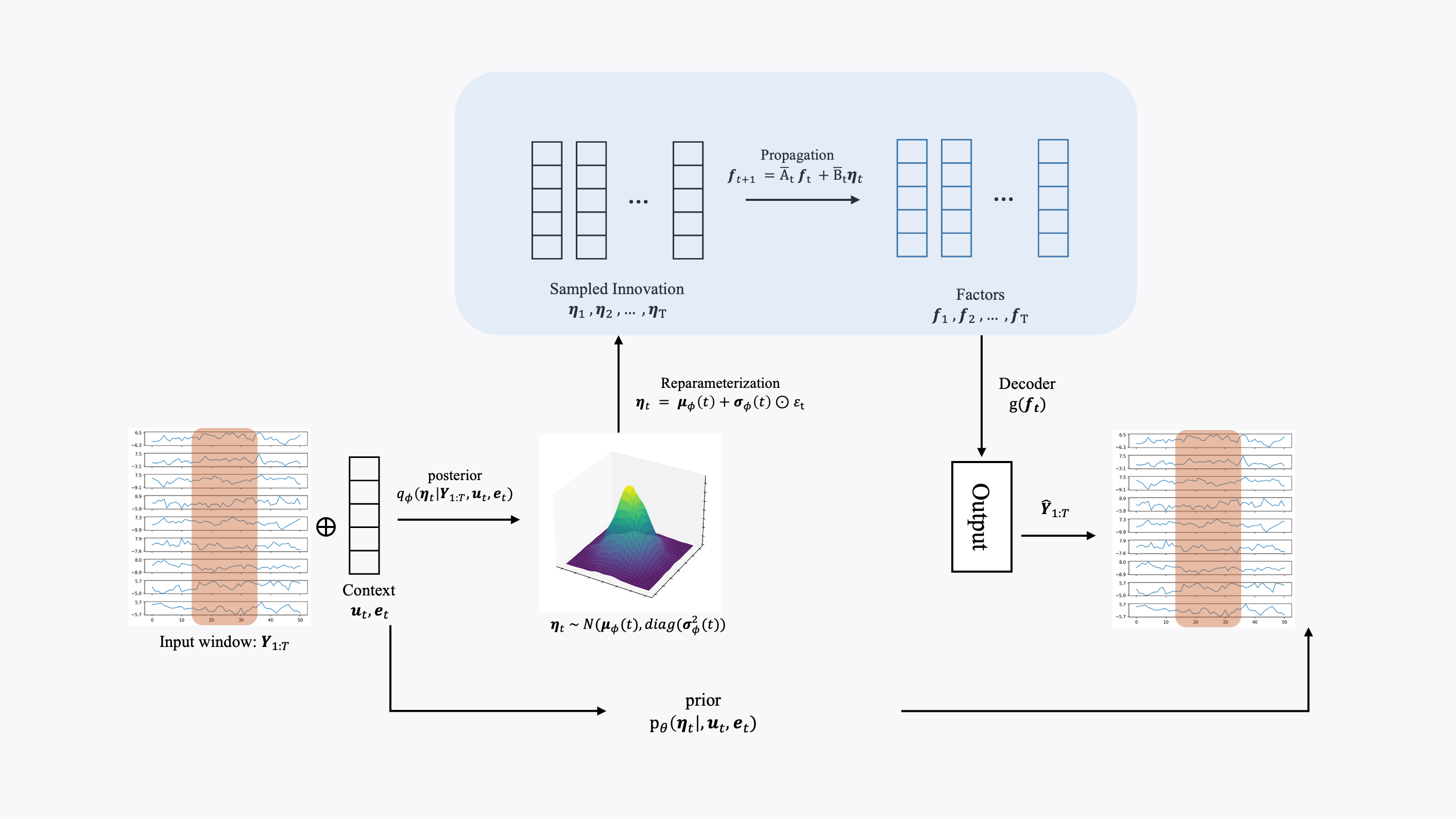
Innovations use a conditional exponential-family prior that depends on auxiliary ${\mathbf{u}}_t$ (calendar, covariates) and a regime embedding ${\mathbf{e}}_t$. The regime embedding is a deterministic soft mixture ${\mathbf{e}}_t={\sum }_j{\pi }_{t,j}{\mathbf{e}}_j$, with weights ${\mathbf{\pi }}_t=\mathrm{softmax}(\mathrm{RegimeNet}({\mathbf{u}}_t))$ over learnable embeddings—so $({\mathbf{u}}_t,{\mathbf{e}}_t)$ stays a deterministic function of observed context, which is what keeps the iVAE-style auxiliary argument valid. Under enough variation in the natural-parameter map $\mathbf{\lambda }({\mathbf{u}}_t,{\mathbf{e}}_t)$, components of ${\mathbf{\eta }}_t$ are identifiable up to $\mathcal{T}$. Gaussian innovations are the wrong tool for this argument in practice (the closure properties of the Gaussian family let you mix coordinates back together), so the implementation uses non-Gaussian innovations such as Laplace.

Dynamics are linear and diagonal: ${\mathbf{f}}_{t+1}={\bar{A}}_t{\mathbf{f}}_t+{\bar{B}}_t{\mathbf{\eta }}_t$, with ${\bar{A}}_t$ and ${\bar{B}}_t$ formed from the same regime weights ${\mathbf{\pi }}_t$ and each component diagonal. Each factor coordinate then depends only on its own history and its own innovation component, so the innovation-level ambiguity class $\mathcal{T}$ transfers unchanged to factor trajectories—a small propagation lemma that fails as soon as the dynamics mix factors or the innovations are Gaussian. AR($p$) dependence fits the same picture via standard companion-form stacking.

Observations come from ${\mathbf{y}}_t=g({\mathbf{f}}_t)+{\mathbf{\epsilon }}_t$ with an injective MLP decoder and fixed-scale noise. Training is standard variational inference: infer innovations, roll the dynamics forward, maximize the ELBO along the Markov structure (reconstruction minus KL to the innovation prior).

What I looked at

The experiments are organized around the three concrete things partial identifiability is supposed to buy you: faithful factor recovery, well-defined interventions, and no collapse in forecast quality.

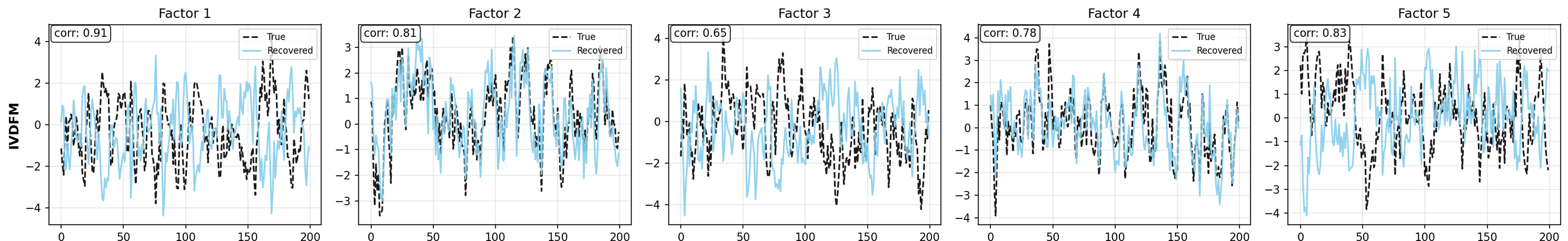
Synthetic factor recovery. On a dynamic DGP (AR dynamics driven by innovations, $T=200$, $N=20$, $r=5$, ten seeds), iVDFM gave the highest mean correlation (MCC $\approx 0.65$) and trace-$R^2$ ($\approx 0.82$) versus DDFM, iVAE, VAE, and DFM. On a static iVAE-style DGP, plain VAE was the strongest baseline and iVDFM merely matched iVAE on MCC. The dynamic-vs-static gap is where the identification signal lives: temporal innovation structure is what iVDFM exploits, so it is the regime where the mechanism is active.

Synthetic interventions. On synthetic SCMs, $do$-interventions on innovation components give model-implied impulse responses that we can compare against ground truth (IRF-MSE, sign accuracy, IRF correlation). On the base (linear) and regime SCMs, IRF errors stay bounded and sign and correlation are workable; on the chain SCM—whose dynamics violate the diagonality assumption—IRF-MSE roughly doubles and sign/correlation fidelity drops. That is exactly the failure mode the propagation lemma predicts: cross-factor interactions break the carry-through of $\mathcal{T}$, so chain-style structures point to richer transition models as the natural relaxation.

Forecasting. On ETTh1/2, ETTm1/2, and Weather at horizons 96–720, probabilistic scores (CRPS and standardized MSE) put iVDFM in the same neighborhood as iTransformer, TimeMixer, TimeXer, and DDFM—competitive on CRPS, not always best on MSE. The lesson is narrow: the innovation-level constraints used to obtain partial identifiability do not destroy distributional forecast quality on these benchmarks; they also do not turn iVDFM into a forecasting specialist.

A small qualitative case study

Beyond synthetic checks and forecast tables, two real panels make the “loadings stay portable across runs” story concrete.

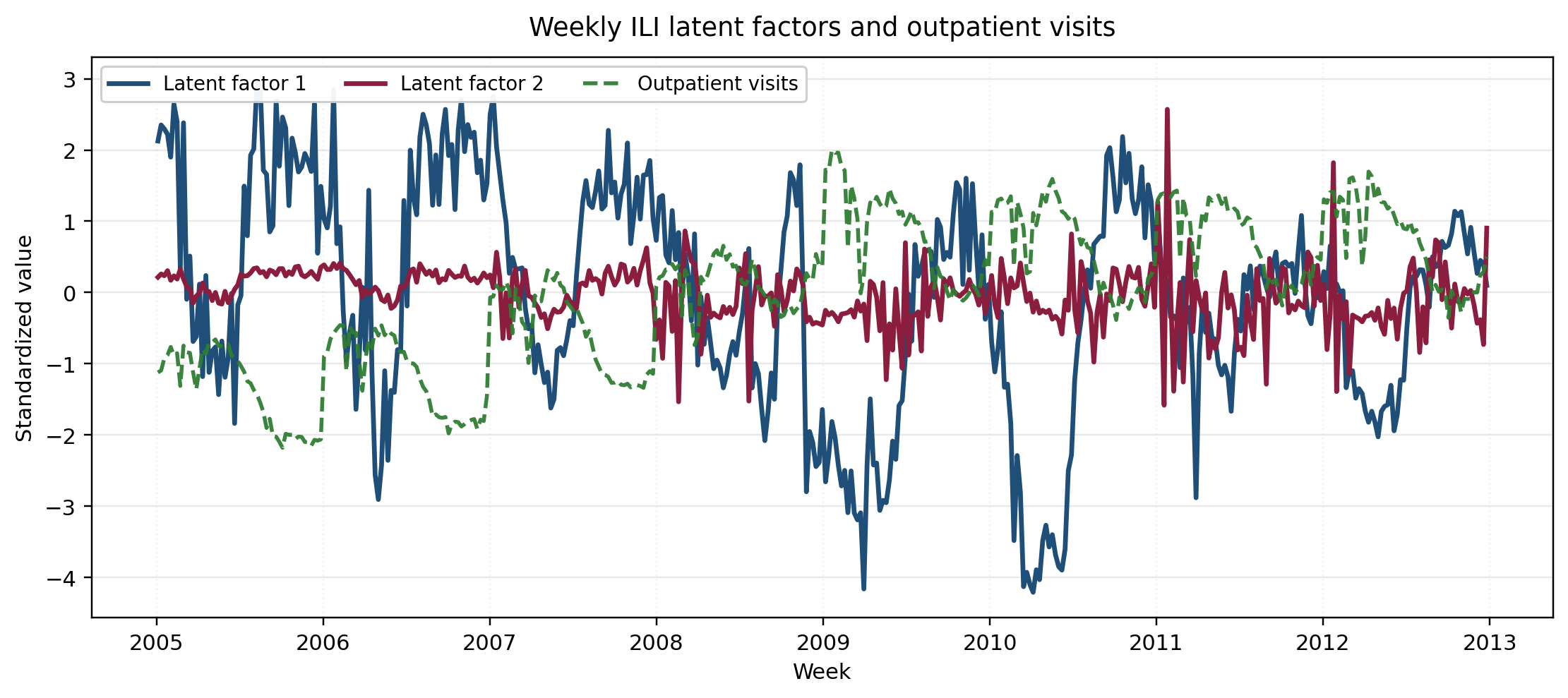
On daily exchange rates for AUD, JPY, CAD, CNY, NZD against USD, two factors ($r=2$) separate a broad market-wide USD component (loading $\approx 0.85$–$0.94$ on the freely moving rates and weak on CNY) from a secondary re-pricing direction with moderate negative loadings on the same currencies. On weekly influenza-like-illness surveillance, the same setup yields one coordinate that moves with shared epidemic burden (strong negative correlations with both ILI rates and outpatient visits) and a second, weaker coordinate that captures utilization-linked residual variation. The point of partial identifiability here is operational: under $\mathcal{T}$, the burden axis stays attachable to the same series across retraining, so dashboards and downstream rules do not need to re-learn which coordinate corresponds to which quantity after each refit.

Caveats and takeaway

If you only need a good number on one benchmark horizon, a forecast-first model is usually simpler to ship. iVDFM is for settings where you also care whether the latent axes are more than a rotating embedding, and where you might later connect latents to regimes or shocks in factor-model language. That only pays off when auxiliaries actually move the innovation prior enough to identify, when non-Gaussian innovations are acceptable, and when diagonal dynamics plus fixed-scale observation noise are not wildly wrong assumptions—none of which is automatic. The chain-SCM result is a useful reminder: as soon as the true dynamics couple factors, the propagation lemma loses its bite and the residual ambiguity grows.

Bottom line: multivariate series can be modeled with shocks and states in mind, not only with next-row prediction. iVDFM is one variational approach in that direction, with partial identifiability up to $\mathcal{T}$ as the main thing it adds over a Gaussian DFM or a generic VAE. In my runs, synthetic checks were useful for understanding behavior, benchmark forecasting was competitive but not consistently top, and the qualitative panel applications give the kind of loadings story that survives retraining. Treat the method as problem-dependent, not as a general replacement for simpler forecasters.

References

1. iVDFM — Chang, M., & Kim, J.-Y. Conditionally Identifiable Latent Representation for Multivariate Time Series with Structural Dynamics.

2. Dynamic factor models — Stock, J. H., & Watson, M. W. (2002). Macroeconomic Forecasting Using Diffusion Indexes. Journal of Business & Economic Statistics, 20(2), 147–162.

3. iVAE / identifiable latents — Khemakhem, I., Kingma, D., Monti, R., & Hyvärinen, A. (2020). Variational Autoencoders and Nonlinear ICA: A Unifying Framework. AISTATS.

4. ICA / non-Gaussianity — Hyvärinen, A., Karhunen, J., & Oja, E. (2001). Independent Component Analysis. Wiley.

5. Deep dynamic factors — Andreini, P., Izzo, C., & Ricco, G. (2020). Deep Dynamic Factor Models. Working paper.

6. Causal representation — Schölkopf, B., et al. (2021). Toward Causal Representation Learning. Proceedings of the IEEE, 109(5), 612–634.