←All posts

What works for forecasting macro economic series with deep learning?

Macro data is awkward for deep learning: a short history, many missing values, and series that arrive at different frequencies. I ran seven model families on the data behind a real-time nowcast of Korean output and investment to see which of them cope. The short answer is that it depends on the target, and the rest of this post is about why.

What the data is like

Macro series give you very few time steps. There are no decades of daily points, so overfitting is the default failure. The setup was the data of a real-time nowcasting pipeline for Korea, the kind the New York Fed runs for the United States: dozens of series on employment, prices, surveys and rates, and two targets, all-industry output and equipment investment.

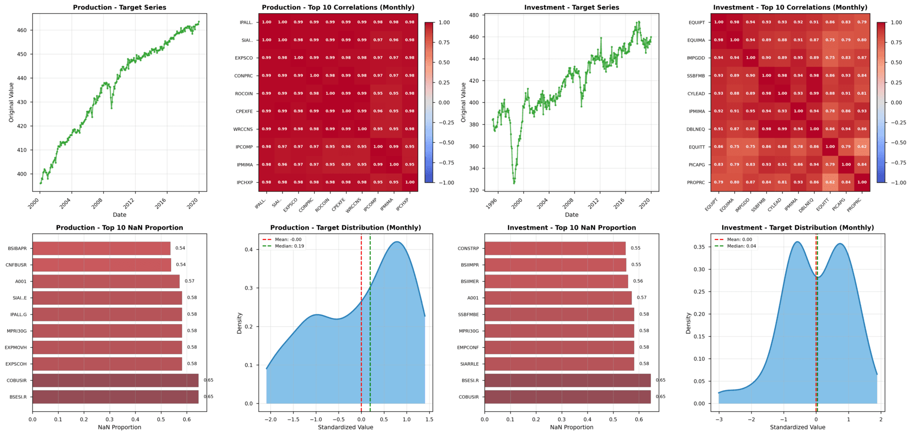
The targets sit at high levels and barely move from one period to the next, the output index especially, so there is limited signal to learn from. The inputs are highly correlated with each other. Some series are weekly, others monthly, and many values are missing, often because they have not been released yet. Models that handle missing data inside the model, which is what state-space and factor models do, start with an advantage. Everything else needs the gaps filled first.

What worked and what did not

Seven models in three families: three attention models (TFT, PatchTST, iTransformer), one mixed-frequency model (TimeMixer), and three state-space models (a dynamic factor model, its deep variant DDFM, and Mamba). All were evaluated the same way, with one-step-ahead forecasts updated each week and aggregated to months, scored by standardised error over the targets.

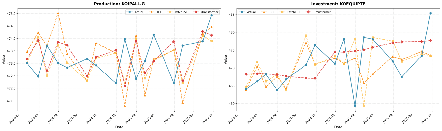
There was no single best model. On the output index, flat and highly correlated, TimeMixer's weekly-to-monthly decomposition had too little variation to work with and did poorly, while on investment, which moves more and has clearer weekly and monthly structure, the same model did well. Among the attention models, iTransformer, which attends across variables rather than across time, was the strongest on output. TFT's attention weights were at least readable: for output they concentrated on corporate bond yields, a news sentiment index and unemployment, and for investment on construction employment and the investment outlook survey.

The classical dynamic factor model, set up like the production nowcast with seven factors, was numerically unstable. As the number of variables grew, the transition matrix had to be held in check with eigenvalue and symmetry constraints to converge at all, which makes the interpretable factors hard to trust. The deep factor model was better behaved, and one change mattered more than any architecture choice: filling the gaps with spline rather than linear interpolation, as the original DDFM paper does, improved it noticeably. Mamba did well on both targets, but its multivariate version was no better than running it on the target alone, so the other series were not helping it.

The practical rule is to match the model to the series and the horizon. State-space models handle missing data and multi-step forecasts consistently, but on short-term accuracy they did not always beat the attention models when the data suited those. For real-time nowcasting, updating the forecast one step at a time beat predicting many steps ahead in one go. The long-horizon runs showed sharp failures at particular horizons when the state was rolled forward without updates.

Limits

One country, one data pipeline, and a short sample, so the conclusions are narrow. What carries over is the shape of the answer rather than any ranking: the data decides which inductive bias helps, interpretability from factor models is only as good as their numerical stability, and for nowcasting the update schedule matters as much as the architecture.

References

1. FRBNY Nowcast — Bok, B., Caratelli, D., Giannone, D., Sbordone, A., & Tambalotti, A. (2019). The FRBNY Staff Nowcast. Federal Reserve Bank of New York Staff Reports, 897.

2. TFT — Lim, B., Arik, S. Ö., Loeff, N., & Pfister, T. (2021). Temporal Fusion Transformers for Interpretable Multi-horizon Time Series Forecasting. International Journal of Forecasting, 37(4), 1748–1764.

3. PatchTST — Nie, Y., Nguyen, N. H., Sinthong, P., & Kalagnanam, J. (2022). A Time Series is Worth 64 Words: Long-term Forecasting with Transformers. arXiv:2211.14730.

4. iTransformer — Liu, Y., Hu, T., Zhang, H., et al. (2023). iTransformer: Inverted Transformers are Effective for Time Series Forecasting. arXiv:2310.06625.

5. TimeMixer — Wang, S., Wu, H., Shi, X., Hu, T., Luo, H., Ma, L., Zhang, J. Y., & Zhou, J. (2024). TimeMixer: Decomposable Multiscale Mixing for Time Series Forecasting. ICLR.

6. Mamba — Gu, A., & Dao, T. (2023). Mamba: Linear-Time Sequence Modeling with Selective State Spaces. arXiv:2312.00752.

7. Deep Dynamic Factor Models — Andreini, P., Izzo, C., & Ricco, G. (2020). Deep Dynamic Factor Models. Working Paper (v. May 2023).

8. Dynamic factor models — Stock, J. H., & Watson, M. W. (2016). Dynamic Factor Models, Factor-Augmented VARs, and Structural VARs in Macroeconomics. Handbook of Macroeconomics, 2, 415–525. Elsevier.