←All posts

Classifying bird sounds in the field

A recorder left in a forest captures hours of audio. We want a program that listens to it and says which birds are calling, and when. The trick that makes this work is to turn the sound into a picture and let an image model look at it. This post walks through the three steps: what a spectrogram is, why the mel version of it is the one people use, and how a network finds a call in the picture. I worked on this in BirdCLEF in 2025 and 2026, and nothing here is exotic.

Sound as a picture

A microphone measures air pressure tens of thousands of times a second, so a recording is a very long list of numbers: the waveform. It is a poor input for a model. Two minutes of audio is millions of numbers, and a bird call is a pattern of pitches changing over time, which the waveform does not show directly.

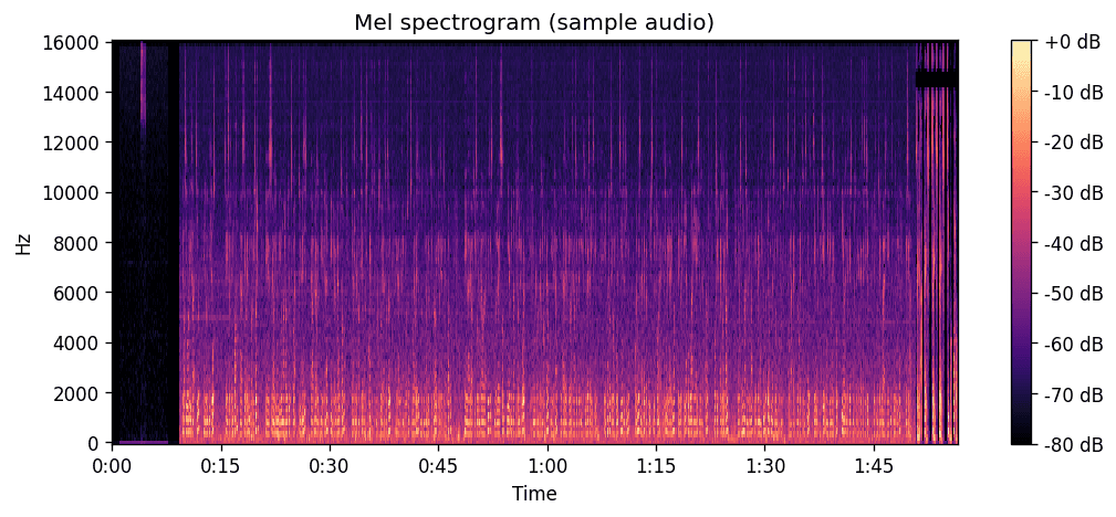
A spectrogram shows exactly that. Cut the audio into short slices, a few hundredths of a second each. For each slice, ask how much energy there is at each frequency, which is what a Fourier transform computes. Then stack the slices left to right. The result is an image: time runs along the horizontal axis, frequency up the vertical axis, and brightness is loudness. A bird call becomes a visible shape. A rising whistle is a stroke going up and to the right, a trill is a row of dots, a croak is a smear across the low frequencies.

Why the mel scale

A plain spectrogram spaces frequencies evenly: the step from 100 to 200 Hz gets the same amount of image as the step from 10,000 to 10,100 Hz. Our ears do not work that way. We hear ratios, so going up an octave sounds like the same move whether it starts low or high. The mel scale re-spaces the frequency axis so that equal distances on it sound like equal steps in pitch: fine resolution at the low end, coarser at the top. The usual formula is

with $f$ in hertz. In practice you keep a few hundred mel bands, and you take the logarithm of the loudness too, because hearing is logarithmic in volume as well as in pitch. What comes out is an image whose rows and brightness match how a listener would perceive the sound. A call that is one shape at a low pitch is a similar shape at a high pitch, which makes the patterns easier for an image model to learn.

Finding the bird in the picture

From here it is image recognition. A small convolutional network, I used EfficientNet-B0, learns the shapes that distinguish species the same way it would learn to tell cats from dogs: edges and strokes in the early layers, longer patterns later. Two adjustments make it a sound classifier rather than an image classifier.

First, several birds call at once, so the output is not one label but one probability per species, each answering a yes or no question on its own. Second, we want to know when the call happened, not just that it happened. So the network keeps the time axis all the way through and produces a score for every species at every time frame. An attention step then combines the frames into a single clip-level answer, giving more weight to the frames where something is happening. The frame scores say where; the clip score says what. This arrangement is called sound event detection.

Training uses clips where the species is known. Two augmentations matter a lot: masking out random strips of time or frequency so the network cannot rely on one feature, and mixing two clips together so it learns that calls overlap, because in the field they always do. At inference time you slide a window along the recording and average the overlapping predictions.

What makes it hard in practice

Training clips are clean: one bird, recorded close. Field recordings are not: several species at once, wind, insects, and long stretches of nothing. A model that is nearly perfect on clean clips loses a lot on real soundscapes. In my case the AUC went from 0.99 on held-out clips to 0.73 on labeled field recordings. The usual fix is to let the model label the field recordings itself and retrain on its confident guesses, and to validate on recordings from the same places the model will be used. That is where most of the work goes, but the three steps above are the foundation everything else is built on.

References

1. Mel scale — Stevens, S. S., Volkmann, J., & Newman, E. B. (1937). A scale for the measurement of the psychological magnitude pitch. Journal of the Acoustical Society of America, 8(3), 185–190.

2. EfficientNet — Tan, M., & Le, Q. V. (2019). EfficientNet: Rethinking Model Scaling for Convolutional Neural Networks. ICML. arXiv:1905.11946.

3. Attention-based sound event detection — Kong, Q., Cao, Y., Iqbal, T., Wang, Y., Wang, W., & Plumbley, M. D. (2020). PANNs: Large-Scale Pretrained Audio Neural Networks for Audio Pattern Recognition. IEEE/ACM Transactions on Audio, Speech, and Language Processing, 28, 2880–2894.

4. Data — BirdCLEF 2025 and BirdCLEF+ 2026, Kaggle.